In this exercise we will apply a stochastic approach to analyzing our predictive model. We will utilize both the parameter estimation and gaussian fields methods and generate probabilistic capture zones.
Before continuing,
1) Launch GMS and open the predictive/particle tracking model you created in case study #4.
2) Save the project under a new name.
We will begin by turning on the stochastic option.
1) Open the Global Options dialog.
2) Change the Run option to Stochastic.
First, we will run a stochastic simulation using the parameter randomization approach. We will randomize recharge zones. If you subdivided your recharge polygon into zones and already parameterized them, you should continue to the "Setting up the Parameter Values" section. If you did not subdivide your recharge into zones, you will need to create some zones before continuing.
If you need to create recharge zones:
1) Select your recharge coverage.
2) Double-click on your recharge polygon and make a note of the recharge value you are using.
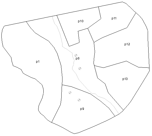
3) Using the Create Arc tool, use Figure 1 as a guide and create a set of interior arcs to subdivide your recharge coverage into a set of polygonal zones. Don't worry about getting the arcs in the exact location; this is just an example. You may wish to come up with your own set of polygons.
4) Select the Build Polygon command. Select each polygon to make sure that the polygons were built correctly.
Figure 1. Suggested Recharge Zones.
Next, we will parameterize the recharge. If your model already had recharge zones and you have already parameterized the recharge zones as part of your calibration exercise, you can continue to the next step.
1) Assign a unique name and enter a unique key value in the recharge field for each of your recharge polygons. If you are using the same recharge polygons you had in your predictive model, be sure to write down the starting value for each of your recharge zones. You will need to enter these later.
2) Select Map->MODFLOW.
3) Open the Parameters dialog.
4) Select the Initialize from Model command. You should see a new set of recharge parameters appear.
To set up the parameter values:
1) Turn on the Stochastic Randomize toggle for each of the recharge parameters.
2) Enter a starting/mean value for your recharge parameters.
a) If you are using your original recharge parameters/polygons from your calibrated model, you should already have your optimal values listed. Leave these values and go to the next step.
b) If you created new recharge zones as part of this exercise, enter the optimal recharge value you used for the single recharge polygon as the mean value for each of your new recharge parameters.
3) Turn OFF the Log Xform option for each of the recharge parameters.
3) In the bottom of the parameters dialog, change the Stochastic option to Random Sampling.
4) Change the Number of instances value to 50. (this is for illustration purposes only as part of this exercise - you will want to use more model runs than this)
5) Change the Std. deviation value to 0.0015 for all parameters.
6) Exit the dialog.
We are ready to run the model.
1) Save and run the model.
2) Exit the model wrapper windows and view the solution. Step through the each of the folders to view the solutions.
Now we can perform a quick probabilistic capture zone analysis using our stochastic solution.
1) Right-click on the folder containing the stochastic solution and select Risk Analysis.
2) Select Probabilistic capture zone analysis and select Next.
3) Select the Stop in cells with weak sinks option.
4) In the section labelled Tracking duration, be sure to select the Specified duration option and enter a travel time in days appropriate to the problem you are working on.
5) The rest of the options should be OK for our case. This will generate a single particle at the water table surface for each cell and will do a separate capture zone for each well. Select Finish.
When the analysis is finished, you should see contours of capture zone probability. If you look in the solution folder, you will see one data set for each of your four wells. Each of these data sets represents probability of capture. Note the overlap of the capture zones for wells G and H with the Beatrice and W.R. Grace properties.
Now we will do a second stochastic simulation using Gaussian fields. We will generate Gaussian fields for hydraulic conductivity. The fields will be conditioned to our optimized K values at the pilot points, but will simulate random heterogeneity between the points.
Before continuing,
1) Delete the stochastic solution folder from the previous run in the Project Explorer.
2) Save the project under a new name.
Next, we will use the FIELDGEN utility to generate our Gaussian fields.
1) In the Project Explorer window, select the 2D scatter point set corresponding to your pilot points, and make sure the data set corresponding to your optimized K values is selected.
2) Open the Gaussian Simulation Options dialog from the Interpolation menu.
3) Double-check the upper right portion of the dialog to make sure the proper scatter point set and data set are selected.
4) Change the Number of realizations to 10. (again, you will want to use more than this in your final analysis - this is for testing purposes only)
5) Turn on the Truncate to specified range option and set the upper and lower bounds to a set of values that are consistent with your optimized K values (0.1 to 200 for example - do not make the min value lower than your lowest pilot point value!). You may even need to make your lower limit higher than the lowest value in your optimized K values in order to make your stochastic solution stable. This requires some experimentation.
6) Make sure that the Condition to scatter points and Calculate mean from scatter points options are both selected.
7) Do NOT turn on log interpolation. I think you get better results in this case with regular interpolation.
8) Click on the Edit Variograms button and create a model variogram. In order to keep your model realizations somewhat close to your calibrated solution, you need to use a really small value for the contribution and a large value for the range. To start, try something like: nugget=10, contribution=100, range=5000.
9) Select the Run Gaussian Simulation command from the Interpolation menu. This will take a few minutes to run.
When the simulator finishes, you should see a folder of data sets on the 3D grid. Turn on contours and select each of the data sets to review.
Next we will change the parameter options so that the K array uses the Gaussian fields we just generated.
1) Open the Parameters dialog.
2) Change the K parameter from pilot points to constant and enter a mean other than zero (2 for example) so that you don't get a warning about the mean being outside the min-max range.
3) Turn on the Use multiplier arrays toggle.
4) In the Multiplier column, change the option to Mult. Arrays.
5) Click on the button in the Data Set/Folder column and select the folder of gaussian arrays we just generated.
For your recharge parameters, you have two options: you can randomize them as we did above or you can make them constant and only vary the K values using the Gaussian arrays.
Save and run your model and review the results. Keep tweaking the Gaussian options and repeat the field generation process until most of your instances are stable and you are comfortable with the results. At this point you can increase your number of model instances, re-run MODFLOW, and then perform your stochastic analysis.