Case Study #4 - Particle Tracking
In this exercise we take the completed predictive model and prepare it for particle tracking analysis.
Loading the Project
Before continuing,
1) Launch GMS and open the predictive model you created in case study #3. Or if you did case studies 4 or 5, use the model resulting from those exercises.
2) Save the project under a new name.
Importing the Site Boundaries
In order to ensure that we will be comparing apples to apples and oranges to oranges, we will import a shapefile containing the Beatrice/Riley and W.R. Grace property boundaries.
1) Right-click to download the properties.zip file.
2) Unzip the file.
3) Right-click on the GIS Layers object in the GMS Project Explorer and select the Add Shapefile Data... command.
4) Select the properties.shp file from the folder containing the unzipped shape file contents.
At this point, the polygon boundaries should appear. You may need to turn off your color-fill contours or adjust the transparency of your contours in order to see the polygons.
Setting up MODPATH
Before continuing, we need to do some initialization with MODPATH.
1) If you can't see the MODPATH menu, right-click on the Grid item in the Project Explorer and turn on the Show MODPATH Menu toggle.
2) Select the MODPATH|Porosity command to bring up the porosity array editor.
Note that the default value for porosity = 0.3. This will have a direct effect on your travel times. This is a reasonable default, but you may choose to adjust it. If you do so, be prepared to defend/justify the value you choose.
3) Select the MODPATH|Zone Code Array command.
Note that the default zone code = 1. We can use zone codes to color our output (pathlines) based on where the particles begin or end. We will assign one zone code to wells G and H and other to the two industrial wells.
5) Select the cells containing wells G and H and click on the Properties icon  .
.
6) Change the MODPATH Zone Code to 2.
7) Use the down arrow in the mini-grid display to switch to layer 2 and repeat for the two well instances for G and H in layer 2.
8) Repeat the previous steps to change the zone code for the industrial wells to 3.
9) Switch back to layer 1.
Note: If you prefer, you can use a different zone code for each of the wells.
Forward Tracking from W.R. Grace
We are now ready to do some particle tracking. To begin we will do forward tracking from the W.R. Grace property. We will select the cells contained within the property in layer 1 and create a set of particles on the top of the water table surface and track the particles forward in time.
1) Zoom in around the W.R. Grace polygon on the east side of the model.
2) Make sure the Select Cell tool is active and select the Edit|Select with Poly command.
3) Start at one of the corners of the polygon and click on each of the corners of the polygon while following a loop (clockwise or counter-clockwise). When you get to the end of the loop, double-click on the starting point.
4) Select the MODPATH|Generate Particles at Selected Cells command. You can either use one particle per cell (the default) or increase the number of particles per cell. Note that the particles are generated on the water table surface by default.
At this point you should see some pathlines appear. You may need to zoom out to see the entire pathlines.
5) Right-click on the new particle set and change the name ("wr-grace" or something).
If your pathlines reach wells G and H, you may wish to vary the color based on where the paths end using the zone codes.
6) Select the MODPATH|Display Options command.
7) Change pathline color option to Ending Code.
8) In the Zone code colors section, turn off the Auto compute colors option and select a set of colors for each of the three zones [OPTIONAL].
Note that the default tracking option is to track all particles until they reach a final destination. We can look at the travel times by selecting the particles/pathlines.
9) Select the Select Particles tool  .
.
10) Drag a box around all of the particles in the W.R. Grace polygon.
Look at the travel times at the bottom of the GMS window. The travel times are shown in days.
We can also compute pathline corresponding precisely to our 14.5 year time period.
11) Double-click on the particle set and change the options so that you are tracking for 14.5 years (5297 days).
Backward Tracking from Wells G and H
Next, we will create a new particle set and do backward tracking from wells G and H.
1) Double-click on the Particle Sets folder and create a new particle set.
a) Rename the particle set to "wells g-h" or something.
b) Change the tracking direction to Backward.
c) Change the duration to 5297 days.
2) Select the two cells containing wells G and H.
At this point, we could use the Select Particles at Cells command, but that will create a single ring of cells around the middle elevation of the cell. We want to have more control on how the particles are distributed in the cells containing the wells.
3) Select the MODPATH|Generate Particles at Cells command.
4) Change the Distribute particles option to On cell faces and turn on the More Options toggle.
5) Play with the settings to distribute particles over the four vertical cell faces. You may wish to do something like what is shown in Figure 1.
6) Repeat for the instances of Wells G and H in layer 2.
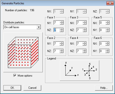
Figure 1. Particle Distributions on Wells G and H.
Conclusion
At this point you can continue to experiment with the particle tracking options. Adjust the particle placement, porosity, display options, etc. The Beatrice property can be treated in a similar fashion. If you performed a transient or stochastic analysis you should perform a particle tracking analysis on those solutions as well.