[Page 6] |
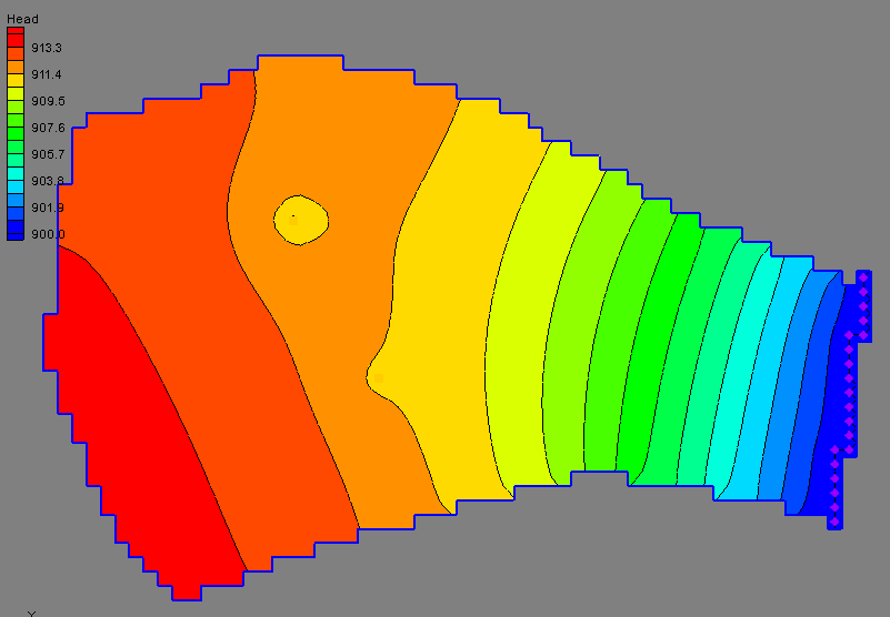
19. (calibration) The following model represents a small aquifer with two low-output wells. The site is bounded on the right by a river, represented with a specified head boundary. The model consists of one layer with two hydraulic conductivity zones and one recharge zone. The objective of this exercise is to calibrate the model.
Click here to download a zip archive containing a copy of a GMS project file representing a starting point for this problem. Unzip the archive to a directory on a local drive. Open the page.gpr project in GMS and complete the following exercise. Follow all instructions carefully. Save your model to disk and re-save frequently throughout the exercise.
Click here to download a copy of the solution.
You may use the GMS Help utility with this problem.
Part 1: Import Observation Well Data
a. (2 pts) Create a new coverage called obs wells for the observation well data. Turn on the appropriate attributes. Choose the option to assign the layers by ID.
b. (3 pts) Click here to download a spreadsheet containing a set of observation well data. Open the spreadsheet and copy the contents to the clipboard. Paste the data into GMS to start the Text Import Wizard. Choose the appropriate settings in the wizard to import the data into the obs wells coverage.
c. (1 pt) Change the Obs Head Interval to 0.5 for each of the points.
Part 2: Flow observations
a. (2 pts) Add a flow observation to the river (specified head) boundary on the right side. Double-click on the source-sink coverage and turn on the Observed flow property. Select the specified head arc on the right and enter an observed flow value = -800 m^3/day. Enter an appropriate interval based on the rule of thumb we discussed in class.
b. (1 pt) Save and re-run the model to compute the head residuals.
Part 3: Parameter Estimation
a. (3 pts) Parameterize the model input. We will be using the two k zones and the one recharge zone as parameters. Using the hyd cond and recharge coverages, enter a set of key values for the three parameters. Use -100 for the north k zone, -200 for the south k zone, and -300 for the recharge. Map the key values to the grid cells
b. (3 pts) Build your parameters and enter the appropriate set of properties/options for the parameters. Use the following starting values:
HK_100: 1.0
HK_200: 1.0
RCH_300: 0.0003
c. (2 pts) Change to parameter estimation mode and save and run the model.
(Upload instructions and links went here)