[Page 6] |
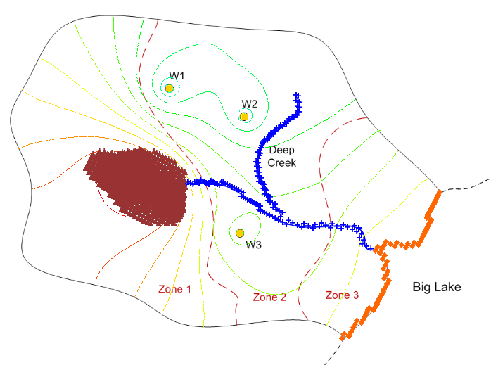
33. This problem is based on a variation of the Big Lake model we built in class this semester:
The objective of this exercise is to parameterize the model, set up particle tracking, and perform a pobabilistic travel time analysis. The question we will be exploring is whether or not the lake is in the 8 year capture zone for the wells.
Click here to download a zip archive of a GMS project.
Click here to download a spreadsheet for making your calculations.
Click here to download a copy of the solution.
Unzip the archive and load the project into GMS. Then do the following:
Paramterize the model.
a. (2 pts) Parameterize the model input using the conceptual model polygons. Paramertize the three K zones and the Recharge using the following key values:
Param Key Value K - Zone 1 -100 4 K - Zone 2 -200 8 K - Zone 3 -300 2 Recharge -400 0.0002 b. (0.5 pts) Save the model as biglake-for and do a run in forward mode. Check to make sure your solution hasn't changed.
Set up particle tracking.
c. (1 pts) Turn on MODPATH and set up a particle tracking analysis. Track backwards from the three wells using 20 particles per well.
d. (1 pts) Change the particle tracking options so that the particle tracking terminates after 8 years.
Mark pathline source by color.
To help us determine which capture zones intersect the lake, we want to change the display of the pathlines based on ending code.
e. (1 pts) Make a copy of the source/sink coverage and change the coverage set up so that you can use it to identify MODPATH zone codes by polygon. Be sure to turn off everything but this setting or you will get a duplicate copy of all sources/sinks in your model.
f. (1 pts) Change the zone code for the lake polygon to 2 and map the coverage to the MODFLOW/MODPATH input.
g. (1 pts) Go into the MODPATH/Particles display options and and turn on the option to color the pathlines by ending code so that the pathlines terminating* in the lake are displayed in a different color. (*technically they are starting in the lake if you consider that we are doing backward tracking).
h. (0.5 pts) Save your project again under the same name.
Set up a stochastic simulation.
i. (0.5 pts) Change the run option to a stochastic simulation.
Go to the Paramaters dialog and:
j. (1.5 pts) Set up all four parameters to be randomized. Do a log transformation on the three K parameters.
k. (1 pts) Use the random sampling option and define 25 model instances.
l. (1.5 pts) For the three K parameters, use standard deviation = 0.3. For the Recharge parameter, use standard deviation = 0.00005.
m. (0.5 pts) Save your model as biglake-stoch and run the simulation.
Determine the probability of capture.
n. (3 pts) Using the spreadsheet, look at each solution and mark a 1 or 0 in the table depending on whether or not any of the pathlines from each of three wells is captured by the lake (or vice versa). Note: If you end up getting zero capture or 100% capture from all wells, you have done something wrong. In this case, make a note on the spreadsheet and enter a random set of zeros and ones so that you can complete the next step.
o. (3 pts) Enter some formulas in the spreadsheet to determine the probability of capture in 8 years for each of the three wells. Save your changes to the spreadsheet. Be sure to upload your spreadsheet with your GMS files (see upload instructions below).
(Upload instructions and links went here)